
Fifty-eight of the seventy-four exported functions, exercised in the
order of a real workflow, on data simulated in the document itself. The
sixteen left out (the inference helpers se_function() and
profile_theta(), qc_phenotypes(),
parentage_check(), competition_strength(),
h_inverse(), read_blupf90_snp(),
estimate_gamma(), dominance_inverse(),
g_epistasis_ad(), g_epistasis_dd(),
g_epistasis_order(), residual_diagnostics(),
mcmc_diagnostics(), and the
_mt/_ar1 twins of
eval_internal()) are documented on their own help pages and
exercised by the test suite. Each chunk runs at build time, so this
walkthrough cannot drift away from the code. The companion vignette
(“from data to breeding value”) tells the story; this one is the tool
bench.
Step 0: simulate a population to work on
simulate_breeding() gene-drops haplotypes, so the
genotypes it emits are consistent with the pedigree it emits: one honest
generator for every example.
library(BreedingR)
s <- simulate_breeding(n_founders = 40, n_generations = 2,
                       offspring_per_generation = 80, h2 = 0.4,
                       n_markers = 200, seed = 7)
str(s, max.level = 1)
#> List of 4
#>  $ pedigree :'data.frame':   200 obs. of  3 variables:
#>  $ data     :'data.frame':   200 obs. of  3 variables:
#>  $ tbv      : Named num [1:200] 1.447 -0.757 -0.439 -0.261 -0.614 ...
#>   ..- attr(*, "names")= chr [1:200] "F001" "F002" "F003" "F004" ...
#>  $ genotypes:List of 2
Step 1: look before estimating
describe(s$data, "y", classes = "cg", pedigree = s$pedigree)
#> Trait 'y': 200 record(s)
#>   mean 10.206, sd 1.0175
#>   quartiles  7.959 /  9.491 / 10.203 / 10.805 / 13.193
#>   3 record(s) outside the Tukey fences [7.52, 12.78]
#>   class cg: 3 level(s), smallest 56, median 64, 0 with a single record
#>   pedigree: 200 animals, 40 founder(s), mean F 0.001875, maximum 0.125
suggest_model(s$data, "y", "id")
#> the shape of the data asks for nothing beyond the base model
Step 2: the pedigree toolbox
p <- pedigree(s$pedigree)      # topological order + Meuwissen-Luo (1992) inbreeding
head(p, 3)
#> Pedigree with 3 animals, 3 founder(s)
#> Mean F 0, maximum 0, 0 animal(s) with F > 0
#>     id sire dam F
#> 1 F001   NA  NA 0
#> 2 F002   NA  NA 0
#> 3 F003   NA  NA 0
ai <- a_inverse(s$pedigree)    # Henderson's (1976) sparse A^-1, as triplets i/j/x/n
str(ai[c("i", "j", "x", "n")])
#> List of 4
#>  $ i: int [1:674] 1 4 19 29 39 47 76 96 113 2 ...
#>  $ j: int [1:674] 1 1 1 1 1 1 1 1 1 2 ...
#>  $ x: num [1:674] 3 0.5 0.5 0.5 0.5 -1 -1 -1 -1 3 ...
#>  $ n: int 200
a22_inverse() takes 1-based positions in the topological
order of pedigree():
gid <- s$genotypes$ids[141:200]
a22i <- a22_inverse(s$pedigree, geno = match(gid, p$id))
dim(a22i)
#> [1] 60 60
A pedigree whose third column holds the MATERNAL GRANDSIRE is
declared, never guessed: read as a dam, the grandsire would enter with
weight 1/2 where the grandsire rules give 1/4 (Mrode and Pocrnic, 2023,
secs. 3.6 and 3.7), and no check downstream could see it.
sire_mgs() declares it, the declaration travels to every
fitter, and a third column named mgs that was not declared
is an error:
bulls <- data.frame(id = c("s1", "s2", "s3", "s4"), sire = c("0", "0", "s1", "s3"),
                    mgs = c("0", "0", "s2", "s2"))
pedigree(sire_mgs(bulls))                  # s4: F = 1/16 through the grandsire s2
#> Sire / maternal-grandsire pedigree with 4 animals, 2 founder(s)
#> Mean F 0.015625, maximum 0.0625, 1 animal(s) with F > 0
#>   id sire mgs      F
#> 1 s1   NA  NA 0.0000
#> 2 s2   NA  NA 0.0000
#> 3 s3    1   2 0.0000
#> 4 s4    3   2 0.0625
Step 3: fit the base animal model, read everything out of it
fit <- model(y ~ cg + animal(id), s$data, s$pedigree)
fit
#> AI-REML fit of 'y'
#>   converged in 5 iteration(s), relDelta 3e-09, Newton decrement 6.53e-20, 0.001 s
#>   -2logL 199.7822977
#>   200 record(s), 203 column(s) in the equations
#>   fixed column(s) removed for linear dependence: cg=g1
#>
#>      component estimate std_error  share correlation
#>    var(animal) 0.416329  0.153150 0.3998
#>  var(residual) 0.625017  0.115851 0.6002
#>
#> fixed effects (implicit intercept; dropped columns are zero; compare by contrast):
#> intercept     cg=g3     cg=g2
#> 10.053836  0.157695  0.270621
summary(fit)
#> AI-REML fit of 'y'
#>   -2logL 199.7822977
#>
#>      component estimate std_error  share correlation
#>    var(animal) 0.416329  0.153150 0.3998
#>  var(residual) 0.625017  0.115851 0.6002
#>
#> fixed effects (implicit intercept; dropped columns are zero; compare by contrast):
#> intercept     cg=g3     cg=g2
#> 10.053836  0.157695  0.270621
#>
#> share: each variance or covariance over the phenotypic variance of its trait,
#> covariances included, the same denominator as h2(); in an animal model the
#> var(animal) row is h2, in a sire model h2() is four times the var(sire) row.
#> A covariance BETWEEN traits, a correlation parameter such as
#> rho(residual), and every row of a model with indirect() have no share.
#> correlation: each covariance over the square root of the two variances it links.
#> For a standard error of either, se_function(fit, function(th) ...) applies the
#> delta method over 2 AI^-1; near a boundary use profile_theta().
coef(fit)
#>   var(animal) var(residual)
#>     0.4163289     0.6250168
round(h2(fit), 3)                           # simulated truth: 0.4
#> [1] 0.4
h2() takes the numerator by name and divides by the
phenotypic variance of the trait: the variances and covariances, never a
correlation parameter such as the rho(residual) of
model_ar1(). In an animal model it is the
share of var(animal) in the printed table.
The fixed effects travel in the same solution vector, named
term=level. The parametrization is the implicit intercept
with dropped columns at zero, so a table from another convention (the
book’s, BLUPF90’s) agrees only on CONTRASTS between levels:
coef(fit, effects = "fixed")                # the same vector as fit$b
#>  intercept      cg=g3      cg=g2
#> 10.0538358  0.1576951  0.2706208
e <- ebv(fit)                               # named vector, all pedigree animals
acc <- accuracy(fit, s$pedigree)            # with the (1+F) in the denominator
round(cor(e[names(s$tbv)], s$tbv), 2)       # against the simulator's own truth
#> [1] 0.76
summary(acc)
#>    Min. 1st Qu.  Median    Mean 3rd Qu.    Max.
#>  0.6644  0.6947  0.7043  0.7156  0.7316  0.8034
head(solutions(fit, s$pedigree), 3)         # id, ebv, se, acc, sorted by ebv
#>         id      ebv        se       acc
#> 194 G2_074 1.192297 0.4650242 0.6932424
#> 157 G2_037 1.155299 0.4660570 0.6915745
#> 1     F001 1.128142 0.4455174 0.7233587
Step 4: the formula markers, one by one
Repeated records ask for a permanent environment;
random() is the iid effect for litter or batch; a
missing-value code leaves the likelihood via
missing_code=:
d3 <- s$data[rep(1:nrow(s$data), each = 2), ]
d3$y <- d3$y + rnorm(nrow(d3), 0, 0.5)
d3$y[1] <- -999
d3$lot <- sample(sprintf("lot%02d", 1:20), nrow(d3), TRUE)
f4 <- model(y ~ cg + random(lot) + animal(id) + pe(id), d3, s$pedigree,
            missing_code = -999)
round(f4$theta, 3)
#>   var(random)   var(animal)       var(pe) var(residual)
#>         0.000         0.473         0.619         0.282
A random() with fewer than five levels warns that its
variance is barely determined; three lots, or a litter numbered by
parity, would.
The full maternal model of Mrode and Pocrnic (2023, Eqn 8.1): direct
and maternal genetic share ONE covariance matrix via
group=, and there is ONE permanent environment, the dam’s,
which carries her non-additive maternal genetics as well.
d5 has two records per animal, so a second
pe() on the animal itself is identifiable here too; on one
record per animal it would BE the residual. Two pe() in one
model must be NAMED:
d5 <- d3
d5$dam <- s$pedigree$dam[match(d5$id, s$pedigree$id)]
d5 <- d5[d5$dam != "0", ]
f5 <- model(y ~ cg + animal(id, group = "g") + maternal(dam, group = "g") +
              pe(id, nome = "pe_animal") + pe(dam, nome = "pe_dam"),
            d5, s$pedigree, missing_code = -999)
names(f5$theta)
#> [1] "var(animal)"          "cov(maternal,animal)" "var(maternal)"
#> [4] "var(pe_animal)"       "var(pe_dam)"          "var(residual)"
The reaction norm is rn() over a basis you build with
legendre(); h2_curve() and plot()
then read h2 along the gradient, and h2() refuses the fit,
because here the heritability is a function of the gradient and not one
number. The pe(id) beside the norm needs repeated records:
with one record per animal it IS the residual, and the fit says SINGULAR
and names the two. So the example reuses the two records per animal of
d3, each at its own THI:
d6 <- d3
d6$thi <- runif(nrow(d6), 55, 80)
d6 <- cbind(d6, legendre(d6$thi, order = 1, limits = c(55, 80)))
f6 <- model(y ~ cg + rn(id, base = c("phi0", "phi1")) + pe(id), d6, s$pedigree,
            missing_code = -999)
head(h2_curve(f6, limits = c(55, 80), points = 5))
#>       x        va        h2
#> 1 55.00 0.7119527 0.4500155
#> 2 61.25 0.5822518 0.4009000
#> 3 67.50 0.4844079 0.3576239
#> 4 73.75 0.4184211 0.3247272
#> 5 80.00 0.3842914 0.3063544
plot(f6, limits = c(55, 80))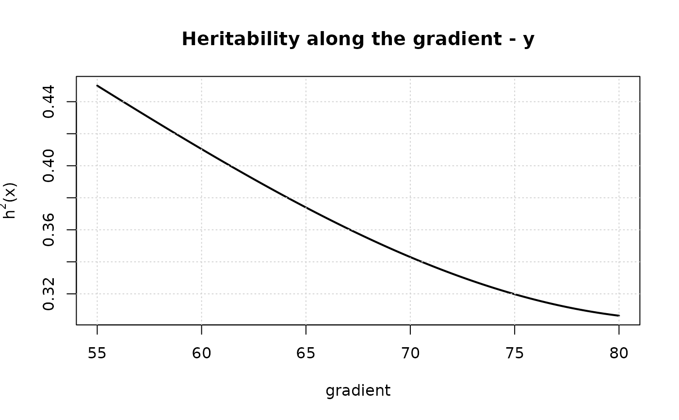
The indirect genetic effect (the associative model of Muir & Schinckel, 2002) marks the PEN MATES in the incidence; direct and indirect share a group so their correlation is estimated:
d7 <- s$data
d7$penc <- rep(sprintf("p%03d", 1:50), length.out = nrow(d7))
f7 <- model(y ~ cg + animal(id, group = "g") + indirect(id, pen = "penc", group = "g"),
            d7, s$pedigree)
round(f7$theta, 3)
#>          var(animal) cov(indirect,animal)        var(indirect)
#>                0.399               -0.022                0.017
#>        var(residual)
#>                0.588
The share column of this fit is blank: each record
carries the indirect effects of its n - 1 pen mates, so its
phenotypic variance depends on the pen size. h2() takes
that size, n, and the relationship between mates,
r, and divides by the phenotypic variance of Bijma, Muir
and Van Arendonk (2007); t2() returns the variance of the
total breeding value A_D + (n - 1) A_S, the ratio T2 and
the direct heritability, with delta-method standard errors:
round(h2(f7, n = 4), 3)
#> [1] 0.385
t2(f7, n = 4)
#>   n r   var_tbv    var_p        t2 h2_direct     se_t2 se_h2_direct
#> 1 4 0 0.4160145 1.037377 0.4010253 0.3850995 0.2270326    0.1221109
Every pen here holds 4 animals taken across generations, and the fit
separates the three components. That is the design’s doing, not the
fitter’s (Cantet and Cappa, 2008): with pens of one size built from two
full-sib families, the data identify only two combinations, the variance
of the total breeding value and va - 2 cov + vs, and the
fit says SINGULAR, names the components and gives them NaN standard
errors.
Real pens are unequal, and with a coefficient of 1 per mate the
social sum grows with the pen size. dilution = d scales
every mate’s entry to (n_i - 1)^(-d) (Bijma, 2010):
d = 0 is the book’s plain sum and the default,
d = 1 the mate mean, and the choice between regimes is a
small grid of d compared on -2logL, which
stays comparable because only the incidence changes. Here the social
effect is planted as the mate MEAN, and the comparison says so:
d8 <- s$data
d8$penc <- sprintf("q%02d", rep(1:50, rep_len(c(2, 3, 6, 9), 50)))[seq_len(nrow(d8))]
sv <- setNames(rnorm(nrow(d8)), d8$id)        # one social value per animal
d8$y <- d8$y + vapply(seq_len(nrow(d8)), function(i) {
  mates <- setdiff(d8$id[d8$penc == d8$penc[i]], d8$id[i])
  if (length(mates)) mean(sv[mates]) else 0 }, 0)
f7d0 <- model(y ~ cg + animal(id, group = "g") +
                indirect(id, pen = "penc", group = "g", dilution = 0),
              d8, s$pedigree)
f7d1 <- model(y ~ cg + animal(id, group = "g") +
              indirect(id, pen = "penc", group = "g", dilution = 1),
              d8, s$pedigree)
round(c(d0 = f7d0$neg2logl, d1 = f7d1$neg2logl), 1)  # the smaller names the regime
#>    d0    d1
#> 247.2 234.6
The residual of the associative model inherits the same group-size
heterogeneity, var(e_i) = s2_ED + (n_i - 1)^(1 - 2d) s2_ES
(Bijma, 2010), with d read from the formula’s
indirect() term. indirect_residual() estimates
the ratio k = s2_ES / s2_ED by profile REML, each candidate
k an exact weighted fit, and returns the whole profile, because with one
record per animal the data pins the slope s2_ES much better
than the ratio (its help page says what is and is not identified):
ir <- indirect_residual(y ~ cg + animal(id, group = "g") +
                          indirect(id, pen = "penc", group = "g", dilution = 1),
                        d8, s$pedigree, k_max = 2, n_grid = 4, tol_k = 0.05,
                        verbose = FALSE)
round(c(k = ir$k, s2_ED = ir$s2_ED, s2_ES = ir$s2_ES), 3)
#>     k s2_ED s2_ES
#> 2.000 0.502 1.003
associative_matrix() writes the same residual as an
exact covariance, one row per record, for a kernel() term:
the block of a pen of n is
(n - 1)^(-2d) [I + (n - 2) J], and a pen of 2 is the
identity:
associative_matrix(c("a", "a", "a", "b", "b"), id = paste0("x", 1:5), dilution = 1)
#>      1    2    3 4 5
#> 1 0.50 0.25 0.25 0 0
#> 2 0.25 0.50 0.25 0 0
#> 3 0.25 0.25 0.50 0 0
#> 4 0.00 0.00 0.00 1 0
#> 5 0.00 0.00 0.00 0 1
#> attr(,"br_associative")
#> [1] 1
A sire model uses sire() when only males carry the
genetic term. Unknown-parent groups enter as metafounders (Legarra et
al., 2015): a parent label with no line of its own, declared with its
gamma:
Step 5: genomics, from files and QC to the single step
read_plink() reads the binary trio (or a .raw); here we
write a tiny .bed by hand so the example carries its own truth:
pref <- file.path(tempdir(), "toy")
codes <- c(`2` = 0L, `1` = 2L, `0` = 3L)                 # 2 bits per genotype
pack <- function(g) { v <- codes[as.character(g)]
  sum(v * 4L^(seq_along(v) - 1L)) }
con <- file(paste0(pref, ".bed"), "wb")
writeBin(as.raw(c(0x6c, 0x1b, 0x01, pack(c(2, 1, 0, 2)), pack(c(0, 0, 1, 1)))), con)
close(con)
writeLines(sprintf("F%d I%d 0 0 0 -9", 1:4, 1:4), paste0(pref, ".fam"))
writeLines(sprintf("1 SNP%d 0 %d A B", 1:2, 1:2), paste0(pref, ".bim"))
read_plink(pref)$m
#>      SNP1 SNP2
#> [1,]    2    0
#> [2,]    1    0
#> [3,]    0    1
#> [4,]    2    1
qc_genotypes() filters animals and markers by call rate,
markers by MAF and (optionally) HWE, and reports what each filter
removed: silent filtering is how panels lose the markers that
mattered.
q <- qc_genotypes(s$genotypes, min_call_rate = 0.9, min_maf = 0.05)
c(animals = length(q$ids), kept = ncol(q$m), by_call = q$n_call, by_maf = q$n_maf)
#> animals    kept by_call  by_maf
#>     200     200       0       0
The APY core can be chosen by rule: apy_core_select()
counts the eigenvalues of G that explain 98% of its trace (Pocrnic et
al., 2016) and draws that many animals at random with a recorded seed,
and apy_core = "auto" does the same inside a fit. On a
genotyped set this small the rule asks for nearly every animal, and the
function warns when one factorization with the core costs more than half
of the exact one; size = overrides the count and the table
of counts is still reported:
gen <- list(ids = gid, m = s$genotypes$m[141:200, ])
core <- apy_core_select(gen, size = 25)
core
#> APY core: 25 of 60 genotyped, explaining 72.0% of G (200 markers, seed 1)
#> eigenvalues of G for 90/95/98/99% of its trace: 41 / 48 / 54 / 56
#> one factorization with this core costs 41.0% of the exact one
The single step is an argument, not a function:
genotypes= upgrades A to H. The inverse of G* is exact by
default, apy_core= uses a global core,
vecchia_k= gives each animal its own conditioning set:
fss <- model(y ~ cg + animal(id), s$data, s$pedigree, genotypes = gen)
fap <- model(y ~ cg + animal(id), s$data, s$pedigree, genotypes = gen,
             apy_core = core)
fve <- model(y ~ cg + animal(id), s$data, s$pedigree, genotypes = gen,
             vecchia_k = 25)
round(c(apy = cor(ebv(fss, "animal"), ebv(fap, "animal")),
        vecchia = cor(ebv(fss, "animal"), ebv(fve, "animal"))), 3)
#>     apy vecchia
#>   0.992   0.998
fss$dense_block                             # the k of the k^3 each factorization pays
#>   dense columns
#>      66     203
Without apy_core= the dense block of the factor holds at
least every genotyped animal, and the fill of the pedigree can add to
it.
The standalone inverses expose the same two approximations with their diagnostics (the Mendelian/conditional residual of each animal):
ap <- apy_inverse(gen$m, core = 1:30)
ve <- vecchia_inverse(gen$m, k = 25)
c(min_apy_res = round(min(ap$mendeliano), 3),
  min_vecchia_res = round(min(ve$mendeliano[-1]), 3))
#>     min_apy_res min_vecchia_res
#>           0.586           0.556
Marker effects come out of a single-step fit by backsolving, or
directly by fitting the markers as equations with
snp_blup(), the path that never builds G (theta is GIVEN,
the routine-evaluation flow):
a_hat <- snp_effects(fss, s$pedigree, gen)
fsnp <- snp_blup(y ~ cg + animal(id), s$data, s$pedigree, gen,
                 theta = unname(fss$theta))
round(cor(unclass(a_hat), fsnp$g[!is.na(fsnp$g)]), 3)
#> [1] 1
pegs() is the fast multi-environment route of Xavier and
Habier (2022): no mixed model equations, no relationship matrix, the
effects of one marker for every environment solved together by
randomized Gauss-Seidel. It assumes the residuals of different
environments are independent, which holds when each animal is recorded
in one place; for traits of the same record, model_mt().
Here the herds of the simulated data stand in for environments. It is
ONE trait, so every true correlation is 1; with 60 animals split three
ways the estimates below are noise, which is what pseudo-expectation
gives on data this small (the method needs thousands of animals to pin
r_g down):
Step 6: multi-trait
cbind() on the left, full R0, missingness handled record
by record; rg() reads the genetic correlation:
Step 7: longitudinal data with a serially correlated residual
model_ar1() needs subject= and
time=. When every gap between consecutive records of a
subject is a whole number of one step (days here), rho is
the correlation per step, far$time_step; with continuous
time it is CAR(1), with rho in [0, 1). The component
rho(residual) is the reason this fitter exists:
nlong <- 5
dar <- s$data[rep(1:nrow(s$data), each = nlong), ]
dar$day <- rep(1:nlong, nrow(s$data))
eps <- replicate(nrow(s$data), as.numeric(arima.sim(list(ar = 0.5), nlong, sd = 0.6)))
dar$y <- dar$y + c(eps)
far <- model_ar1(y ~ cg + animal(id) + pe(id), dar, s$pedigree,
                 subject = "id", time = "day")
round(far$theta[["rho(residual)"]], 2)
#> [1] 0.5
Step 8: the Bayesian half
gibbs() samples the SAME models; ess() and
geweke_z() are the chain diagnostics (also computed
automatically on the result). With theta_fixed= it samples
only the locations, the mode whose posterior mean must be the BLUP.
prior = chooses the prior of the variances
("jeffreys", the default, "flat",
"uniform_sd" or a proper c(df =, scale =)),
and family = "probit" samples a binary trait on its
liability. summary() gives the posterior quantiles and the
heritability computed draw by draw. chains = 3 runs
independent chains (their seeds come from set.seed(), and
cores = runs them at the same time with the same result),
pools them, and adds rhat(), the rank-normalized split
R-hat of Vehtari et al. (2021):
gb <- gibbs(y ~ cg + animal(id), s$data, s$pedigree,
            n_iter = 2000, burnin = 400, thin = 4, chains = 3)
summary(gb)
#> 3 Gibbs chains for 'y', 1200 kept sample(s)
#>
#>      component    mean      sd    q2.5   q50.0   q97.5  rhat ess_bulk ess_tail
#>    var(animal) 0.45683 0.17138 0.18421 0.43623 0.83630 1.015      181      284
#>  var(residual) 0.62373 0.12170 0.41096 0.61743 0.87431 1.013      294      713
#>  mcse_mean mcse_q2.5 mcse_q50.0 mcse_q97.5     status
#>      0.013     0.013     0.0140      0.025 run longer
#>      0.007     0.012     0.0079      0.012 run longer
#>
#> posterior of the ratio, computed sample by sample:
#>                     ratio  mean     sd  q2.5  q50.0  q97.5  rhat ess_bulk
#>  var(animal) / phenotypic 0.416 0.1234 0.181 0.4156 0.6538 1.016      182
#>  ess_tail mcse_mean mcse_q2.5 mcse_q50.0 mcse_q97.5     status
#>       331    0.0092     0.018     0.0095      0.013 run longer
#>
#> fixed effects, posterior mean (implicit intercept; compare by contrast):
#>       term      mean       sd
#>  intercept 10.049561 0.154455
#>      cg=g3  0.152141 0.157087
#>      cg=g2  0.269705 0.165966
#>
#> convergence: run longer (var(animal): R-hat 1.015 with no chain set apart (disagreement 0.89 in location, 0.99 in scale): R-hat^2 is about 1 + 2M/ESS even at convergence (bulk-ESS 181), so more draws bring it down; bulk-ESS 181, tail-ESS 284, below 300 (100 per chain); and 2 more); mcmc_diagnostics() has the full table
round(c(ess = ess(gb$chain_samples[[1]][, "var(animal)"]),
        geweke = geweke_z(gb$chain_samples[[1]][, "var(animal)"]),
        rhat = rhat(sapply(gb$chain_samples, function(m) m[, "var(animal)"]))), 3)
#>    ess geweke   rhat
#> 73.330  2.901  1.015
Step 9: selection decisions
idx <- selection_index(list(y = ebv(fit, "animal"),
                            y2 = ebv(fmt, "animal", trait = "y2")),
                       weights = c(y = 2, y2 = 1))
head(idx, 3)
#>     F001   G2_074   G2_037
#> 7.232769 6.844100 6.669325
drift <- rank_drift(ebv(fit, "animal"), ebv(fss, "animal"), top = 50)
c(spearman = round(drift$spearman, 3), retention = drift$retention)
#>  spearman retention
#>     0.981    47.000
Step 11: selection signatures
fst() needs two or more groups; roh() finds
runs of homozygosity, here with a planted 60-marker run, which comes
back as an island:
s2 <- simulate_breeding(n_founders = 40, n_generations = 1,
                        offspring_per_generation = 40, h2 = 0.4,
                        n_markers = 200, seed = 99)
sc <- fst(rbind(s$genotypes$m, s2$genotypes$m),
          groups = rep(c("A", "B"), c(nrow(s$genotypes$m), nrow(s2$genotypes$m))))
summary(sc$fst)
#>      Min.   1st Qu.    Median      Mean   3rd Qu.      Max.
#> -0.004408  0.029392  0.119492  0.180756  0.279586  0.743027

mroh <- s$genotypes$m[1:30, ]
mroh[1:10, 51:110] <- 2                       # the planted run
rr <- roh(mroh, min_snp = 30)
c(F_ROH_planted = round(mean(rr$animal$f_roh[1:10]), 2),
  island_peak = max(rr$marker$freq_roh))
#> F_ROH_planted   island_peak
#>     0.3100000     0.3333333
Step 12: studies, timing, and the exposed internals
mc_study() repeats simulate-and-refit (cold starts, by
the package’s own rule); benchmark_fit() refuses fewer than
three replicates and checks they returned identical numbers:
m <- mc_study(n_rep = 3, h2 = 0.4, seed = 100, n_founders = 30,
              n_generations = 1, offspring_per_generation = 40)
round(c(mean_h2 = mean(m$h2_est), bias = attr(m, "bias")), 3)
#> mean_h2    bias
#>   0.494   0.094

b <- benchmark_fit(function() model(y ~ cg + animal(id), s$data, s$pedigree), reps = 3)
b
#> 3 run(s): 0.003 / 0.003 / 0.002 s (min 0.002, median 0.003, max 0.003)
#>   results identical across runs
The internals are exported for the gates, and they double as sparse
tools: the same triplet list i/j/x/n that
a_inverse() returns feeds all three:
ch <- sparse_chol(ai)                        # minimum degree (George & Liu 1989; dense
                                             # nodes set aside as in AMD) + symbolic + factor
x1 <- sparse_solve(ai, rep(1, ai$n))         # SOLVES A^-1 x = 1, so x = A %*% 1: the
                                             # row sums of A, without ever forming A
si <- selected_inverse(ai)                   # A at the factor's pattern (PEV reads this)
round(c(logdet = ch$logdet, x1_first = x1[1]), 3)
#>   logdet x1_first
#>  110.904    4.000
inv_pd(matrix(c(4, 1, 1, 3), 2))             # dense positive-definite inverse
#>             [,1]        [,2]
#> [1,]  0.27272727 -0.09090909
#> [2,] -0.09090909  0.36363636
br_version()
#> [1] "0.4.0.9000"
br_threads()                                 # OpenMP threads of the dense tail (default 1);
#> $threads
#> [1] 1
#>
#> $available
#> [1] 4
#>
#> $openmp
#> [1] TRUE
#>
#> $lapack
#> [1] FALSE
                                             # any number gives the same bits
And eval_internal() (with _mt and
_ar1 twins) evaluates -2logL by the TWO independent routes
at any theta: the identity every gate in the package leans on.
ev <- eval_internal(y ~ cg + animal(id), s$data, s$pedigree, theta = c(0.4, 0.6))
round(abs(ev$neg2logl - ev$neg2logl_V), 10)
#> [1] 0
Step 13: declared covariances for dominance, epistasis and breed origin
kernel(id, K=) is the marker for a random term whose
covariance matrix is DECLARED rather than derived from the pedigree or
the markers inside the fit. The constructors build the K:
dominance_matrix() is Cockerham’s D from the pedigree, and
here the data gets a planted dominance deviation (variance 0.3) so the
fit has something true to find. Repeated records keep the dominance
separable from the residual; with one record per animal the two are
confounded up to the sib covariances, and the fit runs to a boundary and
says so:
D <- dominance_matrix(s$pedigree)
set.seed(11)
dv <- drop(chol(D + diag(1e-8, nrow(D))) %*% rnorm(nrow(D))) * sqrt(0.3)
names(dv) <- rownames(D)
dk <- s$data[rep(1:nrow(s$data), each = 2), ]
dk$y <- 10 + s$tbv[dk$id] + dv[dk$id] + rnorm(nrow(dk), 0, sqrt(0.6))
fd <- model(y ~ cg + animal(id) + kernel(id, K = D), dk, s$pedigree)
#> Warning: animal(id): 200 of the 200 animals with records of y have more than
#> one record (400 records between them) and the model has no pe(id): the
#> permanent-environment covariance between records of the same animal goes into
#> var(animal), which inflates h2 by more the larger the share of repeated
#> records; add pe(id), the repeatability model
round(fd$theta, 3)                          # planted: 0.3 kernel, 0.6 residual
#>   var(animal)   var(kernel) var(residual)
#>         0.642         0.267         0.610
The fit warns that the animals have two records and no
pe(id). Here the simulation planted no permanent
environment, so the covariance between the records of an animal that is
not additive IS the dominance deviation, and
kernel(id, K = D) takes it. With real data the two compete
for it: add pe(id), and dominance and permanent environment
are then told apart only by the full-sib covariances in D.
The genomic versions build K from markers: g_matrix()
(raw VanRaden G, the book’s: no blend, no A22 adjustment),
g_dominance() (Vitezica’s genomic D),
g_epistasis() (the Hadamard square with its diagonal
averaged to 1), and genomic_inbreeding() (f = 1 - het/N,
fitted as a cov() and read back from fit$b as
the inbreeding depression):
G  <- g_matrix(gen)
GD <- g_dominance(gen)
GE <- g_epistasis(G)
fin <- genomic_inbreeding(gen)
round(c(diag_G = mean(diag(G)), diag_D = mean(diag(GD)),
        diag_AA = mean(diag(GE)), mean_f = mean(fin)), 3)
#>  diag_G  diag_D diag_AA  mean_f
#>   0.981   0.975   1.000   0.602
partial_a() splits A by breed origin (Garcia-Cortes and
Toro’s partial matrices): one matrix per founder breed, one per
segregating pair, plus the breed-fraction table f and the
segregation coefficients h. A row of K that is entirely
zero declares a level with no contribution (a purebred gets no equation
in the other breed’s term), and each matrix goes into its own
kernel():
pedm <- data.frame(animal = c("1", "2", "3", "4", "5"),
                   sire   = c("0", "0", "1", "1", "3"),
                   dam    = c("0", "0", "2", "2", "4"))
pa <- partial_a(pedm, breed = c("1" = "A", "2" = "B"))
pa$f                                        # 3 and 4 are F1; 5 is F2
#>     A   B
#> 1 1.0 0.0
#> 2 0.0 1.0
#> 3 0.5 0.5
#> 4 0.5 0.5
#> 5 0.5 0.5
round(pa$K[["A"]], 2)                       # the A-partial: animal 2 contributes nothing
#>     1 2    3    4    5
#> 1 1.0 0 0.50 0.50 0.50
#> 2 0.0 0 0.00 0.00 0.00
#> 3 0.5 0 0.50 0.25 0.38
#> 4 0.5 0 0.25 0.50 0.38
#> 5 0.5 0 0.38 0.38 0.62
pa$h                                        # only the F2 segregates
#>   A:B
#> 1   0
#> 2   0
#> 3   0
#> 4   0
#> 5   1
Step 14: a categorical trait on the liability scale
model_threshold() fits an ordered categorical trait by
probit on an underlying liability (Gianola and Foulley), residual FIXED
at 1 for identifiability, thresholds in place of the intercept,
components GIVEN via start=. With
estimate = TRUE the same start= is only the
starting point and the components are estimated as the minimum of the
Laplace -2logL the fit reports, known to run low for a binary trait with
few records per level; gibbs(family = "probit") avoids the
Laplace approximation. predict() returns the per-category
probabilities:
dt <- s$data
dt$cat <- as.integer(cut(dt$y, quantile(dt$y, c(0, 0.6, 0.85, 1)),
                         include.lowest = TRUE))
ft <- model_threshold(cat ~ cg + animal(id), dt, s$pedigree, start = 0.35,
                      verbose = FALSE)
round(ft$thresholds, 3)
#>    t1    t2
#> 0.457 1.395
head(ebv(ft), 3)                            # on the liability scale
#>        F001        F002        F003
#>  0.61315244 -0.30598924  0.01157069
round(predict(ft, dt[1:2, ]), 3)            # P(category) per record
#>          1     2     3
#> [1,] 0.362 0.359 0.280
#> [2,] 0.714 0.219 0.066
h2_observed() and h2_liability() are the
Dempster and Lerner conversion between the 0/1 observed scale and the
liability scale: at incidence 0.234 half the heritability is scale, not
biology.
round(c(observed = h2_observed(0.1781, 0.234),
        liability = h2_liability(0.0934, 0.234)), 4)
#>  observed liability
#>    0.0934    0.1781
Step 15: time until failure, with censoring
model_survival() fits the Weibull frailty model
(Kachman); censor= is mandatory because a censored record
is a LOWER BOUND on the failure time, not a missing value. This chunk is
Example 16.1 of Mrode and Pocrnic (length of productive life of 12 cows,
4 censored), and the numbers it prints are the book’s p.291-292. A
covariate that changes during a life enters as elementary records
(entry, stop] of one subject, through
entry = and subject =:
cows <- data.frame(
  cow  = as.character(8:19),
  herd = as.character(c(1,1,1,1,1,1,2,2,2,2,2,2)),
  ysp  = as.character(c(3,4,1,2,3,1,4,1,2,3,4,2)),
  code = c(0,1,0,1,1,1,1,1,0,1,0,1),        # 0 = censored
  lpl  = c(40,47,22,28,50,33,49,29,23,37,35,30))
peds <- data.frame(
  animal = as.character(1:19),
  sire = c(rep("0", 7), "1","1","4","4","5","5","1","1","5","5","4","4"),
  dam  = c(rep("0", 7), "2","3","2","9","3","8","6","7","14","6","7","3"))
fsu <- model_survival(lpl ~ herd + ysp + animal(cow), cows, peds, censor = "code",
                      rho = 1, lambda = 1, sigma2 = 0.4, verbose = FALSE)
round(coef(fsu, "fixed"), 3)                # herd=2 -1.631, ysp -2.346/-3.149/-2.982
#> herd=2  ysp=2  ysp=3  ysp=4
#> -1.631 -2.346 -3.149 -2.982
round(exp(ebv(fsu)[["1"]]), 3)              # relative risk of animal 1: 0.459
#> [1] 0.459
round(predict(fsu, data.frame(herd = "1", ysp = "4", cow = "1"),
              time = 40, type = "survival"), 3)   # S(40) = 0.394
#> [1] 0.394
A covariate that changes along the life enters as elementary records
(entry, stop] of one subject. survival_split()
builds them from one row per subject and one row per change, and
predict(entry =) is the survival over one piece, so the
survival of a life is the product over its pieces:
subj <- data.frame(id = c("a", "b"), time = c(40, 30), event = c(1, 0), ysp = "1",
                   herd = "1", cow = c("1", "2"))
chg <- data.frame(id = "a", at = 20, ysp = "2")
pieces <- survival_split(subj, chg)
pieces
#>   id time event ysp herd cow entry
#> 1  a   20     0   1    1   1     0
#> 2  a   40     1   2    1   1    20
#> 3  b   30     0   1    1   2     0
prod(predict(fsu, pieces[pieces$id == "a", ], time = pieces$time[pieces$id == "a"],
             entry = pieces$entry[pieces$id == "a"], type = "survival"))
#> [1] 4.284783e-05
The rule behind the tour
A new model is almost never a new function: it is a marker inside the
formula of one engine, kernel() being the marker that takes
ANY declared covariance. A sibling fitter exists only when the
mathematics changes: model_mt() (the residual becomes R0),
model_ar1() (the residual gains serial correlation),
gibbs() (the algorithm samples instead of maximizing),
snp_blup() (a fixed-components solver with markers as
equations), model_threshold() (the residual stops being
Gaussian with a free variance), model_survival() (there is
no residual at all: the randomness is the Weibull the linear predictor
scales). Everything else orbits the fit.